
How do machines learn?
Last time, we briefly learned about machine learning. I learned that machine learning largely includes supervised learning, reinforcement learning, and unsupervised learning, and among these, the most commonly used method is the supervised method. So today, we will take a look at how machines learn, using the example of artificial intelligence that predicts science scores using math scores. If you input a student’s math score, we will create a model that learns from the data and predicts the student’s science score. Let’s look at the specific process of how the model learns from the data.
📢 This article focuses on theory rather than practice writing code for supervised learning, so please refer to it before reading.
Select model
When starting machine learning, model selection is one of the important steps. The model determines what type of learning algorithm to use for a given task, and different models are specialized for different tasks.

A model is a function that outputs a value y when an input value x is given. For now, it is simply expressed as y = wx as shown in the image above, but there are many different models in artificial intelligence. However, let’s study the easy and simple first-order function y = wx.
So this time, let’s look at and study a model that predicts the science score (y) when the math score (x) is entered. Then, in the equation, the input value x can be the math score and the output y value can be the science score. And w represents weight. This model is a simple linear regression model in which the input value x multiplied by the weight w produces the output value y. Weights are adjusted during the model learning process and represent the relationship between input and output values. As weights are adjusted during the learning process, the model is optimized to make predictions appropriate for the data.
📢 A little more detail on what weights are
Weight is a parameter that indicates the importance assigned to each input feature in machine learning and neural network models. Weights are adjusted while the model is training and determine how input features affect the output. Weights in linear models are coefficients that are multiplied for each input feature. Taking the example above y = wx as an example, y = w1x1 + w2x2 +… In a multivariate linear regression model such as wnxn, each wi represents the weight for the corresponding input xi.
The role of weights is to determine how input features affect the output. The higher the weight, the more influence the input feature has on the output. As the model is trained, these weights learn the relationship between input and output and are adjusted to make optimal predictions. Weights are adjusted to the data by a learning algorithm, which optimizes the model to produce accurate output for a given input.
Data collection
Once the model has been decided, it is time to collect data. In order to learn a model, a sufficient amount of training data is required. Training data must consist of input data and the correct answer (label or target) for that data. When collecting data, you must consider the quality and diversity of the data.
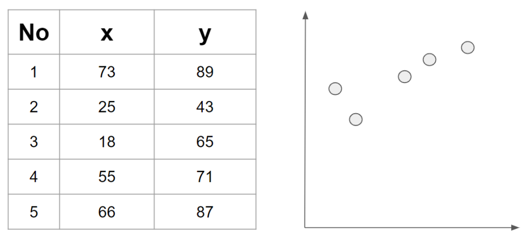
The collected data was expressed in tables and graphs as shown in the image above. In the example above, there are only 5 pieces of data, but in reality, much more data is needed. However, please note that only five pieces of data are displayed for convenience.
Now, let’s take a look at the data above. For student number 1, the math score (x) is 73 points and the science score (y) is 89 points. Similarly, for student number 2, the math score is 25 points and the science score is 43 points. Since supervised learning requires both training data and the correct answer to be provided, in the current situation, the math score (x) is the data to be trained, and the science score (y) is the correct answer (label) that the model should predict.
Training
Generally, when training a model in artificial intelligence, parameters and weights are initially set randomly. This is a technical choice that helps the model learn different patterns.
Weight initialization can affect model performance, and choosing an appropriate initialization method is important. One of the widely used initialization methods is Xavier or Glorot initialization. This method randomly initializes the weights so that the mean is 0 and the variance is a specific value.
Another initialization method is He initialization. This method is effective when used with the ReLU activation function. He initialization randomly initializes the weights so that the mean is 0 and the variance is doubled.
Since the initialization method can affect the model’s performance and learning speed, it is recommended to select an appropriate initialization method depending on the model and data used.
You don’t need to know much about the initialization methods mentioned above, just refer to them as “those things exist.” In the example we will learn today, we will not use the initialization methods mentioned above and will assume that the random value of w, the parameter part in the y = wx part, is 0.1.
Predict
Then, since w is currently 0.1, the model determined above will have the form y = 0.1x. The first task performed in the training phase is to output predicted values from the current model. In other words, the expected science score is output by putting the math scores of 5 people, 73, 25, 18, 55, and 66, in the x value.
y = 0.1x
| No | x | y | ŷ |
| 1 | 73 | 89 | 7.3 |
| 2 | 25 | 43 | 2.5 |
| 3 | 18 | 65 | 1.8 |
| 4 | 55 | 71 | 5.5 |
| 5 | 66 | 87 | 6.6 |
Let’s take a look at the first student’s score. The math score x is 73 points, and the predicted science score is y = 0.1x, so it is 7.3. However, this student’s actual science score is 89 points, which is a whopping 81.7 points different from the predicted science score of 7.3 points. This is a natural result since it is still in the early stages of learning, and this gap will gradually decrease. For reference, the predicted y value is usually expressed as y-hat to distinguish it from the actual y value.
Loss
The next thing to do in the training phase is to calculate the loss. Here, loss refers to the difference between the actual y value and the y value predicted by the model. As we just saw for the first student, his actual science score was 89, but his predicted science score was 7.3. Therefore, the first student’s loss value is 81.7 points. Therefore, it can be said that the current loss value for the first student is very large. Also, in the case of the second student, the actual science score is 43 points, but the predicted science score is 2.5 points, which is a large loss.
Of course, a large loss value is not a good thing. Therefore, the learning goal of the model is to minimize the loss value.
Optimization
The third task to be performed in the training phase is optimization. Optimization is updating parameters so that loss values are reduced. In this training, we set the parameter value to 0.1. But this time, let’s assume it has been modified to 0.3.
y = 0.3x
| No | x | y | ŷ |
| 1 | 73 | 89 | 21.9 |
| 2 | 25 | 43 | 7.5 |
| 3 | 18 | 65 | 5.4 |
| 4 | 55 | 71 | 16.5 |
| 5 | 66 | 87 | 19.8 |
If you look at the y-hat (predicted value), you can see that it is closer to the correct answer than when the parameter was 0.1, but you can see that it is not yet close to the correct answer. In general, when learning a model, it does not end with a single update, but is improved repeatedly and gradually. Therefore, the prediction value calculation, loss calculation, and optimization performed in previous training must be repeated.
In the case of the first student, when the parameter was 0.1, the loss value was 81.7 by calculating y (correct answer) – y-hat (predicted value), but when the current parameter was predicted to be 0.3, the loss value was reduced to 68.1. . However, the loss value is still very large, so it needs to be made smaller.
Therefore, optimization (optimization) must be performed to modify parameters to reduce the current loss value. If you repeat the Predict – Loss – Optimization process like this, the loss value will continue to decrease and get closer to the correct answer. And in this process, w is gradually updated to reduce the loss value.
And if you keep repeating the above process, there comes a point when the loss value no longer decreases. If the loss value no longer decreases, training is stopped.
To summarize, in this example, the model equation was initially set as y = wx, and the w value was continuously updated through training. And the value of w when the loss value no longer decreases will become the final equation of the model. For example, when w is 1.5, if the loss value has not decreased any further, the final equation of the model will be y = 1.5x.
Conclusion
Ultimately, what machine learning means is finding the parameters and weights in the model. Here, parameters refer to the number of functional expressions. In other words, learning a model is ultimately a process of finding the number.
The initial model has undetermined parameters, like a house that only has a shape, but appropriate parameter values are updated through learning. It can be said to be similar to filling in detailed elements such as windows, doors, and chimneys of a house.
In this example of machine learning, a simple model with only one parameter, y = wx, was used. However, recently released models have a very large number of parameters and have a complex structure. Chat GPT-3.5, which is currently gaining popularity, also consists of approximately 175 billion parameters. Most of these super-large artificial intelligence models fall into the field of deep learning.
However, whether the number of parameters is 1 or 1,750, the learning method is not much different from the example learned in this lesson. It’s just that the larger the number of parameters, the more work has to be done compared to the previous example (y = wx) because work has to be done on each parameter.
Therefore, it requires a lot of computation when learning, and it is impossible to train the model without expensive computer equipment.
Lastly, I will summarize and conclude the terms learned through this study.
| keyword | meaning |
| Model | function with parameters |
| Parameter(weight) | Variables that exist inside the model and must be found through learning |
| Loss | Difference between the y value predicted by the model and the actual y value (The smaller the loss, the better. Parameters must be updated to reduce the loss.) |
| Optimization | The process of updating parameters as loss decreases |